How To Plot Columns Of A Matrix In Matlab

MATLAB - Plotting

---

To plot the graph of a function, you need to take the following steps −

• Ascertain x, by specifying the range of values for the variable x, for which the office is to be plotted

• Define the office, y = f(x)

• Call the plot command, every bit plot(x, y)

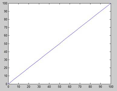
Following example would demonstrate the concept. Let us plot the simple office y = x for the range of values for ten from 0 to 100, with an increment of 5.

Create a script file and type the post-obit code −

x = [0:5:100]; y = x; plot(x, y)        

When you run the file, MATLAB displays the following plot −

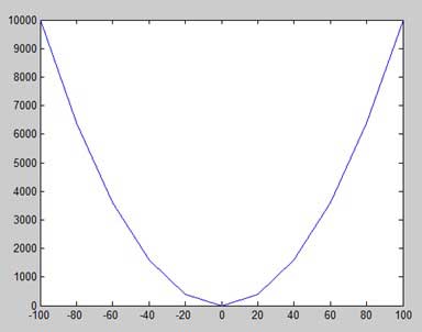
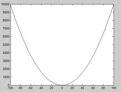
Let us accept one more example to plot the part y = x². In this case, we will draw two graphs with the same function, merely in second fourth dimension, we will reduce the value of increment. Please note that as we decrease the increment, the graph becomes smoother.

Create a script file and type the following code −

x = [1 two 3 4 5 6 vii eight ix 10]; x = [-100:20:100]; y = x.^2; plot(x, y)        

When you run the file, MATLAB displays the following plot −

Alter the code file a picayune, reduce the increase to v −

x = [-100:5:100]; y = x.^ii; plot(x, y)        

MATLAB draws a smoother graph −

Calculation Title, Labels, Grid Lines and Scaling on the Graph

MATLAB allows you to add title, labels along the x-axis and y-axis, grid lines and also to adjust the axes to spruce up the graph.

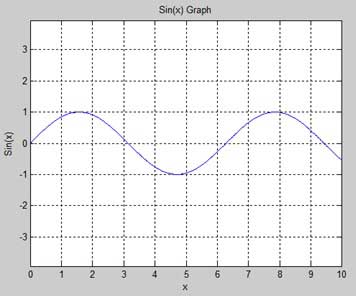
• The xlabel and ylabel commands generate labels along x-centrality and y-centrality.

• The title control allows you to put a title on the graph.

• The grid on command allows you to put the grid lines on the graph.

• The centrality equal control allows generating the plot with the same calibration factors and the spaces on both axes.

• The axis square command generates a square plot.

Instance

Create a script file and blazon the following lawmaking −

x = [0:0.01:10]; y = sin(x); plot(x, y), xlabel('x'), ylabel('Sin(x)'), title('Sin(x) Graph'), grid on, axis equal        

MATLAB generates the following graph −

Drawing Multiple Functions on the Same Graph

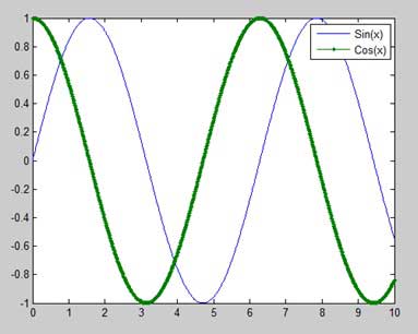
Y'all tin describe multiple graphs on the same plot. The post-obit example demonstrates the concept −

Example

Create a script file and type the post-obit code −

x = [0 : 0.01: 10]; y = sin(x); g = cos(10); plot(ten, y, 10, k, '.-'), fable('Sin(x)', 'Cos(x)')        

MATLAB generates the following graph −

Setting Colors on Graph

MATLAB provides 8 basic colour options for cartoon graphs. The following table shows the colors and their codes −

Code	Colour
w	White
k	Blackness
b	Blue
r	Red
c	Cyan
m	Greenish
m	Magenta
y	Yellow

Example

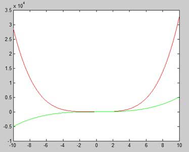
Let us depict the graph of two polynomials

• f(x) = 3x⁴ + 2x³+ 7x² + 2x + 9 and

• m(x) = 5xⁱⁱⁱ + 9x + 2

Create a script file and type the following code −

x = [-10 : 0.01: 10]; y = 3*x.^4 + 2 * x.^3 + 7 * x.^2 + 2 * x + 9; g = v * x.^iii + nine * x + two; plot(ten, y, 'r', ten, thou, '1000')        

When you run the file, MATLAB generates the following graph −

Setting Axis Scales

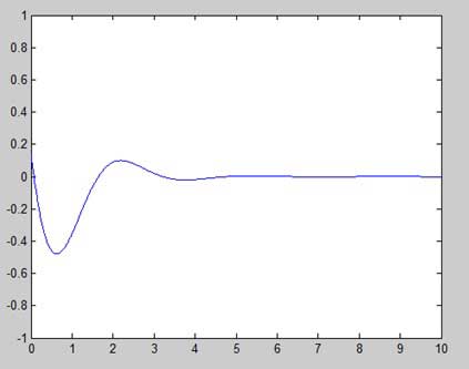
The axis control allows you lot to gear up the axis scales. You can provide minimum and maximum values for 10 and y axes using the axis command in the following fashion −

centrality ( [xmin xmax ymin ymax] )        

The following example shows this −

Instance

Create a script file and type the following lawmaking −

ten = [0 : 0.01: ten]; y = exp(-x).* sin(2*x + three); plot(x, y), axis([0 ten -1 ane])        

When y'all run the file, MATLAB generates the following graph −

Generating Sub-Plots

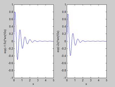
When you create an array of plots in the same figure, each of these plots is called a subplot. The subplot command is used for creating subplots.

Syntax for the command is −

subplot(m, n, p)        

where, m and n are the number of rows and columns of the plot array and p specifies where to put a particular plot.

Each plot created with the subplot control can have its own characteristics. Following case demonstrates the concept −

Example

Let us generate two plots −

y = due east^−i.5xsin(10x)

y = due east^−2xsin(10x)

Create a script file and blazon the following code −

10 = [0:0.01:5]; y = exp(-one.v*10).*sin(10*x); subplot(1,2,ane) plot(10,y), xlabel('x'),ylabel('exp(–1.5x)*sin(10x)'),axis([0 5 -1 one]) y = exp(-two*x).*sin(x*x); subplot(1,2,2) plot(x,y),xlabel('x'),ylabel('exp(–2x)*sin(10x)'),centrality([0 5 -1 i])        

When you lot run the file, MATLAB generates the following graph −

Source: https://www.tutorialspoint.com/matlab/matlab_plotting.htm

Share this post